

Linear regression is the first model most people learn and the one most people stop reading too early. They fit it, report R², and move on. In this article we will do the whole job on a real dataset: fit the model, interpret it, test its assumptions, try a regularised alternative, and then use what the diagnostics tell us to build a much better model.
The data: 1,338 insurance bills#
The Medical Cost Personal dataset (on Kaggle) has one row per person: age, sex, BMI, number of children, smoker or not, US region, and annual medical charges billed by insurance. Charges are what we want to predict.
import pandas as pd

df = pd.read_csv("insurance.csv")
df["charges"].describe()
# mean 13,270   median 9,382   min 1,122   max 63,770
df["charges"].skew()   # 1.52
The mean is well above the median, and the skewness is 1.5. Most people have modest bills and a minority have very large ones. That long right tail will matter later.
One comparison says more than any summary statistic:
df.groupby("smoker")["charges"].median()
# no: 7,345    yes: 34,456
The median smoker is billed almost five times as much as the median non-smoker.
Fitting the model#
Categorical columns need to become numbers. get_dummies with drop_first=True creates one 0/1 column per category except a reference category, which avoids perfectly redundant columns:
import statsmodels.api as sm
from sklearn.model_selection import train_test_split

d = pd.get_dummies(df, columns=["sex", "smoker", "region"], drop_first=True)
X = d.drop(columns="charges").astype(float)
y = d["charges"]
X_train, X_test, y_train, y_test = train_test_split(X, y, test_size=0.2, random_state=42)

ols = sm.OLS(y_train, sm.add_constant(X_train)).fit()
print(ols.summary())
I use statsmodels here rather than scikit-learn because it reports what we need for interpretation: standard errors, p-values and confidence intervals. Keep the column names (pass a DataFrame, not .values), otherwise the summary labels everything x1, x2, x3 and you spend your afternoon counting columns.
Reading every coefficient#
| Term | Coefficient | p-value |
|---|---|---|
| Intercept | −11,930 | < 0.001 |
| age | +257 per year | < 0.001 |
| bmi | +337 per unit | < 0.001 |
| children | +425 per child | 0.006 |
| sex: male | −19 | 0.961 |
| smoker: yes | +23,650 | < 0.001 |
| region: northwest | −371 | 0.490 |
| region: southeast | −658 | 0.223 |
| region: southwest | −810 | 0.131 |
Each coefficient reads the same way: holding all the other variables constant, a one-unit increase in this variable is associated with this change in annual charges. So:
- Each extra year of age adds about $257 a year.
- Each BMI point adds about $337.
- Smoking adds about $23,650, by far the largest effect, and the most precisely estimated one (t = 50.7).
- Sex and region are not statistically significant. Once age, BMI and smoking are known, being male or living in the northwest tells us nothing reliable about charges.
The intercept, −$11,930, is the predicted bill for a zero-year-old with a BMI of zero. It is not interpretable; it exists to put the line in the right place.
Two words of caution. "Associated with" is deliberate: this is observational data, so these are not causal effects. And "not significant" means the data cannot distinguish the effect from zero, not that the effect is proven to be zero.
The model explains 74.2% of the variance in the training data (R²), and on the held-out 20% it scores R² = 0.784, with a typical error (RMSE) of $5,796 and an average absolute error (MAE) of $4,181.
Checking the assumptions#
Linear regression's p-values and confidence intervals are only trustworthy if four assumptions hold, remembered as LINE: Linearity, Independence, Normality of the errors, and Equal variance of the errors. The fastest check is to plot residuals (actual minus predicted) against fitted values. A good model gives a shapeless horizontal band around zero.
Ours does not. Look at the left panel below:
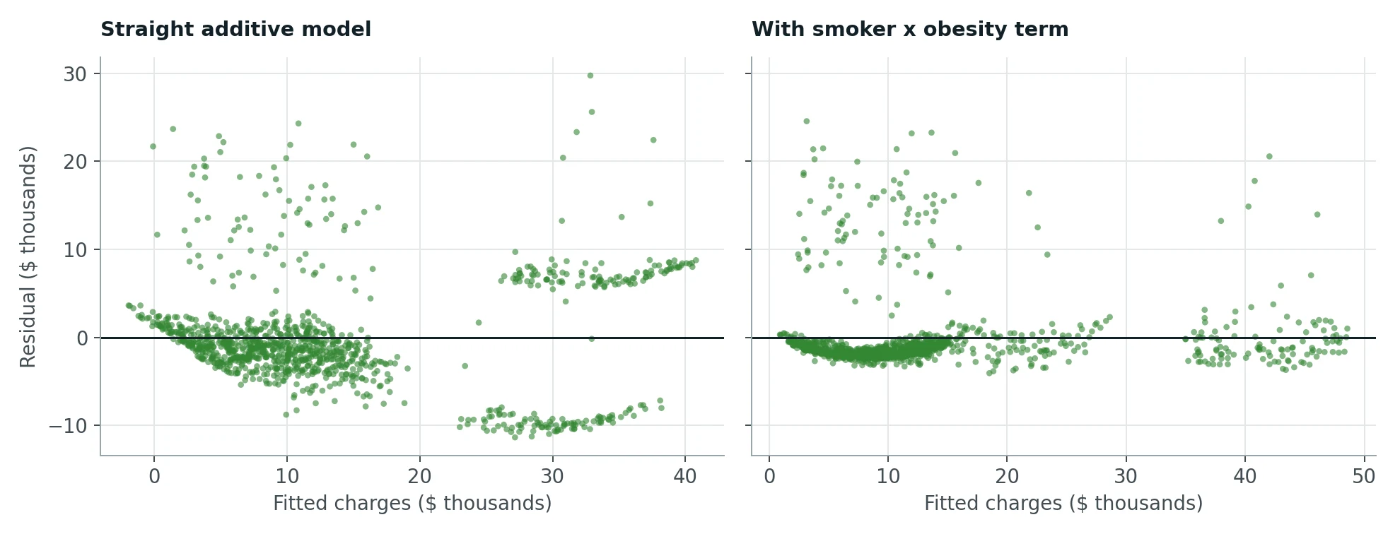
Instead of a cloud, the residuals form distinct bands. There is a group predicted around $25k to $40k whose residuals are about −$10k, and another whose residuals are about +$7k. The model is systematically wrong for whole groups of people. The formal tests agree:
- Normality: Shapiro-Wilk W = 0.894, p ≈ 10⁻²⁶. The residuals are not normal.
- Equal variance: Breusch-Pagan p ≈ 10⁻¹⁶. The spread of the errors changes with the prediction.
- Independence is about how the data was collected. One row per person, with no repeated measurements, is plausibly independent.
When residuals form bands, it usually means the model is missing a variable or an interaction. So what are those bands?
Letting the data explain the bands#
Plot charges against BMI and colour by smoking status:
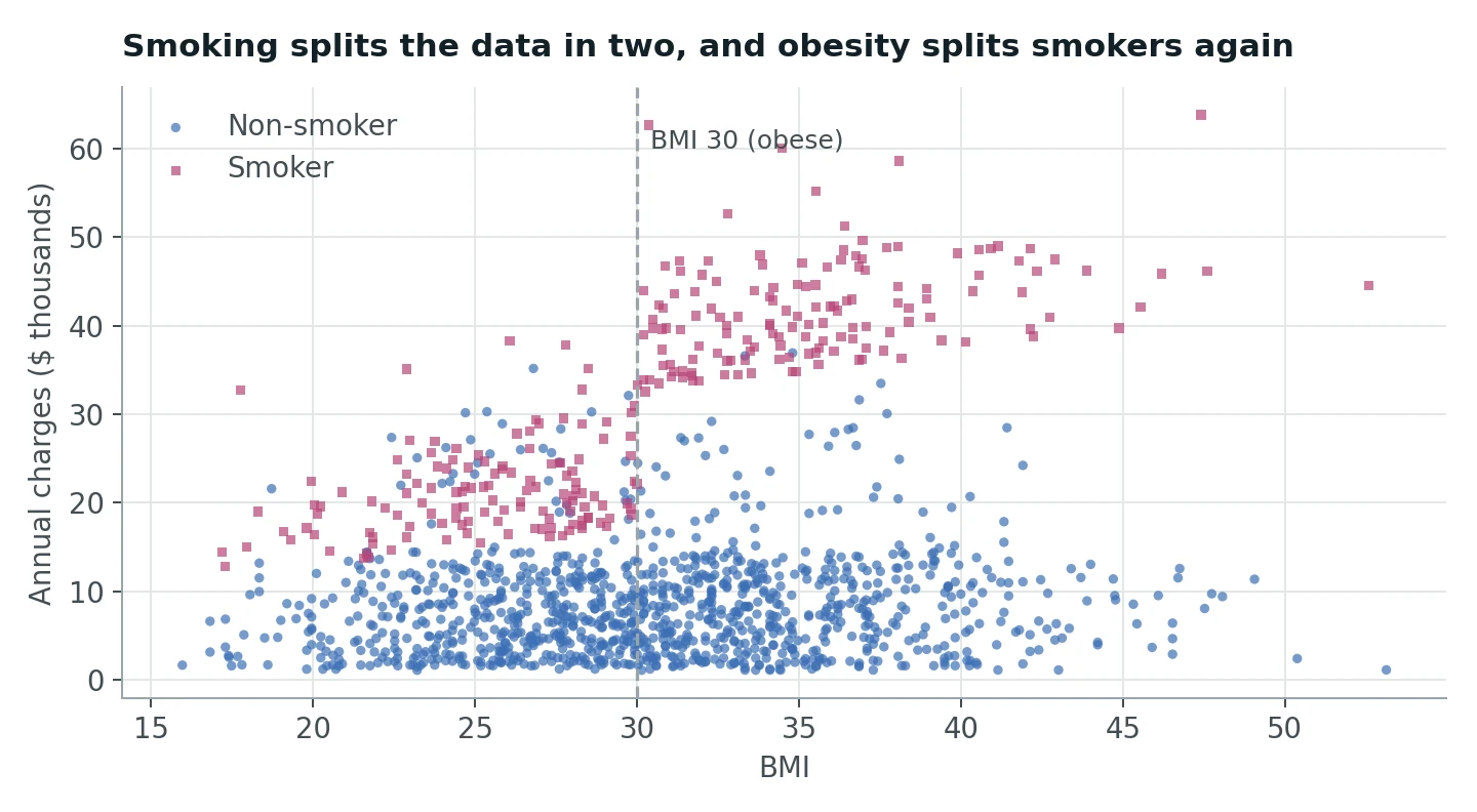
There it is. Non-smokers sit in a low band regardless of BMI. Smokers split in two, with a jump right at BMI 30, the clinical threshold for obesity. A smoker who is obese is billed far more than smoking and obesity would each predict separately.
Our model cannot express that, because it assumes effects add up. The smoking effect is the same $23,650 whether your BMI is 22 or 38. What the data shows is an interaction: the effect of BMI depends on whether you smoke.
The model we should have built#
Add a flag for obesity and a flag for "smoker and obese":
d["obese"] = (d["bmi"] >= 30).astype(float)
d["smoker_x_obese"] = d["smoker_yes"] * d["obese"]
Refit, and the coefficients tell a much clearer story. Smoking alone adds about $13,170. Being an obese smoker adds a further $20,090 on top. Meanwhile the plain BMI coefficient shrinks from $337 to $94: most of what we thought was "BMI raises costs" was really "BMI raises costs for smokers".
The right-hand residual plot above shows the effect: the bands collapse into a tight line near zero. And the numbers:
| Additive model | With interaction | |
|---|---|---|
| Test R² | 0.784 | 0.873 |
| Test RMSE | $5,796 | $4,440 |
| Test MAE | $4,181 | $2,465 |
| 10-fold CV R² | 0.739 ± 0.059 | 0.857 ± 0.042 |
The average absolute error dropped by 41%. We got there not by switching to a fancier algorithm, but by reading the residual plot and asking what it was trying to say. There is still a scattered group of people with much higher bills than predicted (the dots above the band). Nothing in this dataset explains them; they are likely people with a serious illness or accident that year.
A regularised alternative: Lasso#
Back to the original eight features for a moment, because there is another tool worth knowing: Lasso. Lasso is linear regression with a penalty on the size of the coefficients. The penalty strength, λ (called alpha in scikit-learn), is chosen by cross-validation. Its signature behaviour is that it pushes weak coefficients to exactly zero, performing feature selection.
Features must be standardised first so the penalty treats them fairly:
import numpy as np
from sklearn.linear_model import LassoCV
from sklearn.preprocessing import StandardScaler

scaler = StandardScaler().fit(X_train)
lasso = LassoCV(alphas=np.logspace(-4, 4, 80), cv=10, max_iter=5000)
lasso.fit(scaler.transform(X_train), y_train)
lasso.alpha_   # 119.1
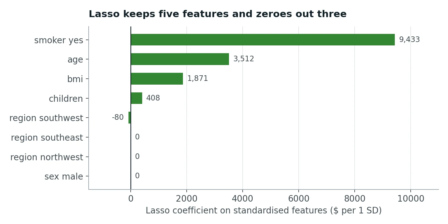
Lasso zeroed out sex and two of the regions, which matches the non-significant p-values from OLS. Because the inputs are standardised, the coefficients are directly comparable: a one-standard-deviation change in smoking status matters about 2.7 times more than one standard deviation of age.
On accuracy, Lasso and OLS are tied: test R² of 0.780 against 0.784, and 10-fold CV R² of 0.739 for both. That is expected. Lasso shines when you have many features, some of them useless or strongly correlated, and not much data. With eight features and 1,070 training rows, there is little overfitting for it to prevent.
Which model when?#
- If someone asks why the model predicts what it does (a doctor, a regulator, an underwriter), OLS with its coefficients, confidence intervals and p-values is the right tool, provided the assumptions roughly hold.
- If you have many candidate features and want a smaller model that predicts well, Lasso does selection and fitting in one step.
- Whatever you choose, the residual plot is not optional. In this dataset it was the difference between R² 0.78 and 0.87.
What to take away#
- Interpret each coefficient as "holding everything else constant" and never forget it is association, not causation.
- Check LINE with a residuals-vs-fitted plot before trusting any p-value.
- Structure in the residuals means the model is missing something. Go find it in the data.
- Interaction terms let the effect of one variable depend on another. Real-world effects often work this way.
- Lasso is a great tool for many-feature problems, but it cannot find an interaction you did not give it.