

Most machine learning models are hard to compute by hand. Naive Bayes is the exception: you can train one with a pencil, and doing it once teaches you more than reading about it ten times. So that is where we start. Then we scale up to a real text classifier in scikit-learn and tune it properly.
The idea in one sentence#
To classify a message, ask: if this message were spam, how likely would these exact words be? Ask the same for "not spam" (usually called ham), weight each answer by how common that class is, and pick the larger.
Written out:
score(class) = P(class) × P(word₁ | class) × P(word₂ | class) × ...
prediction   = the class with the highest score
The "naive" part is treating each word as independent of the others, given the class. That assumption is obviously false ("free" and "prize" appear together in spam far more than chance would predict), and yet the classifier works remarkably well. It turns out you do not need correct probabilities to rank two classes correctly.
A tiny training set#
Six messages, three of each class:
| Message | Label |
|---|---|
| cheap loan offer now | SPAM |
| win cash prize now | SPAM |
| claim free loan today | SPAM |
| team lunch today | HAM |
| project review meeting | HAM |
| lunch with the team | HAM |
We want to classify a new message: "free lunch". Before reading on, guess. "Free" is a spam word here, "lunch" is a ham word. It could go either way.
Step 1: priors#
The prior is just how common each class is. Three of six messages are spam, so:
from collections import Counter

label_counts = Counter(label for _, label in train)
priors = {label: n / len(train) for label, n in label_counts.items()}
# {'SPAM': 0.5, 'HAM': 0.5}
Step 2: word counts#
Count every word inside each class, and count the vocabulary: the number of distinct words across all messages.
word_counts = {"SPAM": Counter(), "HAM": Counter()}
for text, label in train:
    word_counts[label].update(text.split())

total_tokens = {label: sum(c.values()) for label, c in word_counts.items()}
V = len(set(w for c in word_counts.values() for w in c))
# total_tokens = {'SPAM': 12, 'HAM': 10},  V = 17
Step 3: the zero problem#
The natural estimate of P(word | class) is "how often the word appears in that class, divided by the total words in that class". Try it on our message:
| P(free | class) | P(lunch | class) | Score | |
|---|---|---|---|
| SPAM | 1/12 = 0.083 | 0/12 = 0 | 0 |
| HAM | 0/10 = 0 | 2/10 = 0.2 | 0 |
Both scores are zero. "Lunch" never appeared in spam, so the model concludes spam is impossible, and "free" never appeared in ham, so ham is impossible too. One unseen word wipes out all the other evidence, because anything multiplied by zero is zero. On real data, where most words are rare, this would happen on almost every message.
Step 4: Laplace smoothing#
The fix is to pretend we saw every vocabulary word alpha extra times in every class. With alpha = 1 (add-one smoothing):
P(word | class) = (count(word, class) + alpha) / (total_tokens(class) + alpha × V)
ALPHA = 1.0

def likelihood(word, label):
    return (word_counts[label][word] + ALPHA) / (total_tokens[label] + ALPHA * V)

def score(message, label):
    p = priors[label]
    for word in message.split():
        p *= likelihood(word, label)
    return p
Now nothing is ever exactly zero:
| P(free | class) | P(lunch | class) | Score | |
|---|---|---|---|
| SPAM | 2/29 = 0.069 | 1/29 = 0.034 | 0.5 × 0.069 × 0.034 = 0.00119 |
| HAM | 1/27 = 0.037 | 3/27 = 0.111 | 0.5 × 0.037 × 0.111 = 0.00206 |
HAM wins. Why? "Lunch" appears twice in ham, and ham has fewer total words, so its smoothed likelihood (0.111) is much stronger evidence than "free" is for spam (0.069). Smoothing did not decide the answer; it made it possible to have one.
Two practical notes. First, real implementations add logarithms of probabilities instead of multiplying them, because multiplying hundreds of small numbers underflows to zero in floating point. Second, alpha is a hyperparameter. One is a convention, not a law, and we are about to tune it.
Scaling up: a sentiment classifier#
Now a slightly more realistic problem: 60 short product reviews, 30 positive and 30 negative.
"absolutely love this it works perfectly and feels great"      -> pos
"cheap flimsy materials and it broke almost immediately"        -> neg
In scikit-learn, the whole thing is a Pipeline: a vectorizer that turns text into word features, followed by the classifier. Keeping them in one pipeline matters, because it guarantees the vocabulary is learned only from training data during cross-validation. Fit the vectorizer on everything first and you have leaked test words into training.
from sklearn.model_selection import train_test_split, GridSearchCV
from sklearn.pipeline import Pipeline
from sklearn.feature_extraction.text import TfidfVectorizer
from sklearn.naive_bayes import MultinomialNB

X_train, X_test, y_train, y_test = train_test_split(
    texts, labels, test_size=0.30, random_state=42, stratify=labels
)  # 42 train, 18 test

pipe = Pipeline([("vec", TfidfVectorizer()), ("nb", MultinomialNB())])

param_grid = {
    "vec__ngram_range": [(1, 1), (1, 2)],          # words, or words + word pairs
    "nb__alpha": [0.01, 0.1, 0.5, 1.0, 2.0, 5.0],  # smoothing strength
}
grid = GridSearchCV(pipe, param_grid, scoring="f1_macro", cv=4).fit(X_train, y_train)
grid.best_params_   # {'nb__alpha': 0.01, 'vec__ngram_range': (1, 1)}
grid.best_score_    # 0.776
TfidfVectorizer weights each word by how distinctive it is (frequent in this review, rare across reviews). MultinomialNB technically expects counts, but it works well with TF-IDF weights in practice. I tried CountVectorizer too; it reached the same best score (0.776, at alpha=0.5) and the same test accuracy.
Macro-F1 averages the F1 score of each class, so neither class can hide behind the other. On this balanced dataset it tracks accuracy closely, but it is a good habit.
On the 18 held-out reviews, the best model scores 88.9% accuracy and 0.889 macro-F1: 16 right, 2 wrong.
Read the grid, not just the winner#
It is tempting to report best_params_ and move on. Look at the whole grid instead:
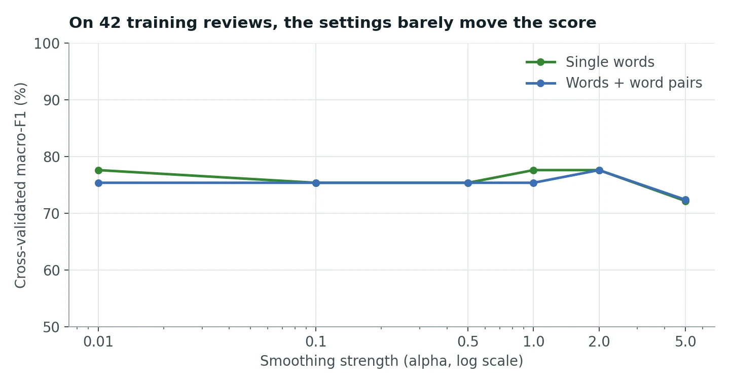
Every setting scores between 0.72 and 0.78. With 42 training reviews split four ways, each validation fold has about 10 reviews, so one review flipping is worth several points. The "winner" won by roughly one review. The honest summary is that for any alpha up to 2, the settings are roughly tied, and very heavy smoothing (alpha=5) starts to hurt because it flattens the difference between words the model has seen and words it has not.
Did word pairs help? No. Adding bigrams never beat single words, and usually did slightly worse. With 42 short reviews, most bigrams ("works perfectly", "stopped working") appear only once or twice. Each one adds a feature with almost no evidence behind it, so the model gets more noise rather than more signal. Bigrams earn their keep on large corpora, where "not good" appears often enough to learn that it is not the same as "good".
What the model learned#
Because Naive Bayes stores a probability for every word in every class, we can ask which words push hardest toward each label:
- Toward positive: works, premium, great, flawlessly, solid, perfectly, impressed
- Toward negative: useless, flimsy, disappointed, broke, terrible, stopped, overpriced
Exactly what you would hope. Now the two mistakes:
- "reliable and beautifully designed I have no complaints", predicted negative. "No" and "complaints" are negative words in isolation. A bag-of-words model has no idea that "no" negates "complaints".
- "misleading the product is nothing like the photos shown", predicted positive. "Misleading" appears nowhere in training, and the rest of the sentence is neutral words that happen to lean positive.
Both errors come from the same place: the model sees words, not meaning. Negation in particular is the classic failure of bag-of-words models, and it is the problem bigrams (on enough data) or modern language models are designed to solve.
What to take away#
- Naive Bayes multiplies a class prior by per-word likelihoods and picks the most probable class.
- Without smoothing, one unseen word zeroes out a class. Laplace smoothing fixes that;
alphacontrols how strongly. - Put the vectorizer and the model in one
Pipelineso cross-validation cannot leak vocabulary. - On a small dataset, differences between hyperparameter settings are often noise. Read the whole grid.
- Naive Bayes is fast, needs very little data, and is easy to inspect. That makes it a strong first baseline for any text problem, even if it is rarely the last model you ship.