

A single decision tree is easy to read and easy to fool. Change a handful of training rows and you can get a noticeably different tree. On the breast cancer data we use below, I trained ten trees on ten random resamples of the same training set and their test accuracy ranged from 88.1% to 93.7%. That instability is the problem random forests were invented to solve.
The idea is almost embarrassingly simple: train hundreds of trees, make each one a little different on purpose, and let them vote.
How a forest makes its trees different#
Two sources of randomness:
- Bootstrap sampling (bagging). Each tree trains on a sample of the training rows drawn with replacement, the same size as the original. Some rows appear twice or three times, and about 37% of rows are left out of any given tree.
- Random feature subsets. At every split, a tree may only consider a random subset of the features (for classification, the square root of the number of features by default). This stops every tree from making the same obvious first split.
Each individual tree is still deep and overfit. But their errors are different, and when you average many independent-ish errors, they largely cancel. The forest keeps the low bias of deep trees while shedding most of their variance.
We will use the Wisconsin breast cancer dataset: 569 tumours, 30 measurements each, 212 malignant and 357 benign. A single fully-grown tree gets 100% on its training data and 92.3% on the test set. A 500-tree forest gets 95.8% on the same test set.
Now to the four questions.
1. How many trees do you need, and can too many hurt?#
Remember those rows each tree never saw? They give us a free validation set. For every training row, collect votes only from the trees that did not train on it. The accuracy of those votes is the out-of-bag (OOB) score, an honest estimate of generalisation without a separate hold-out set.
from sklearn.ensemble import RandomForestClassifier

for n in [10, 25, 50, 100, 200, 400, 800, 1600]:
    rf = RandomForestClassifier(n_estimators=n, oob_score=True, random_state=42, n_jobs=-1)
    rf.fit(X, y)
    print(n, rf.oob_score_)
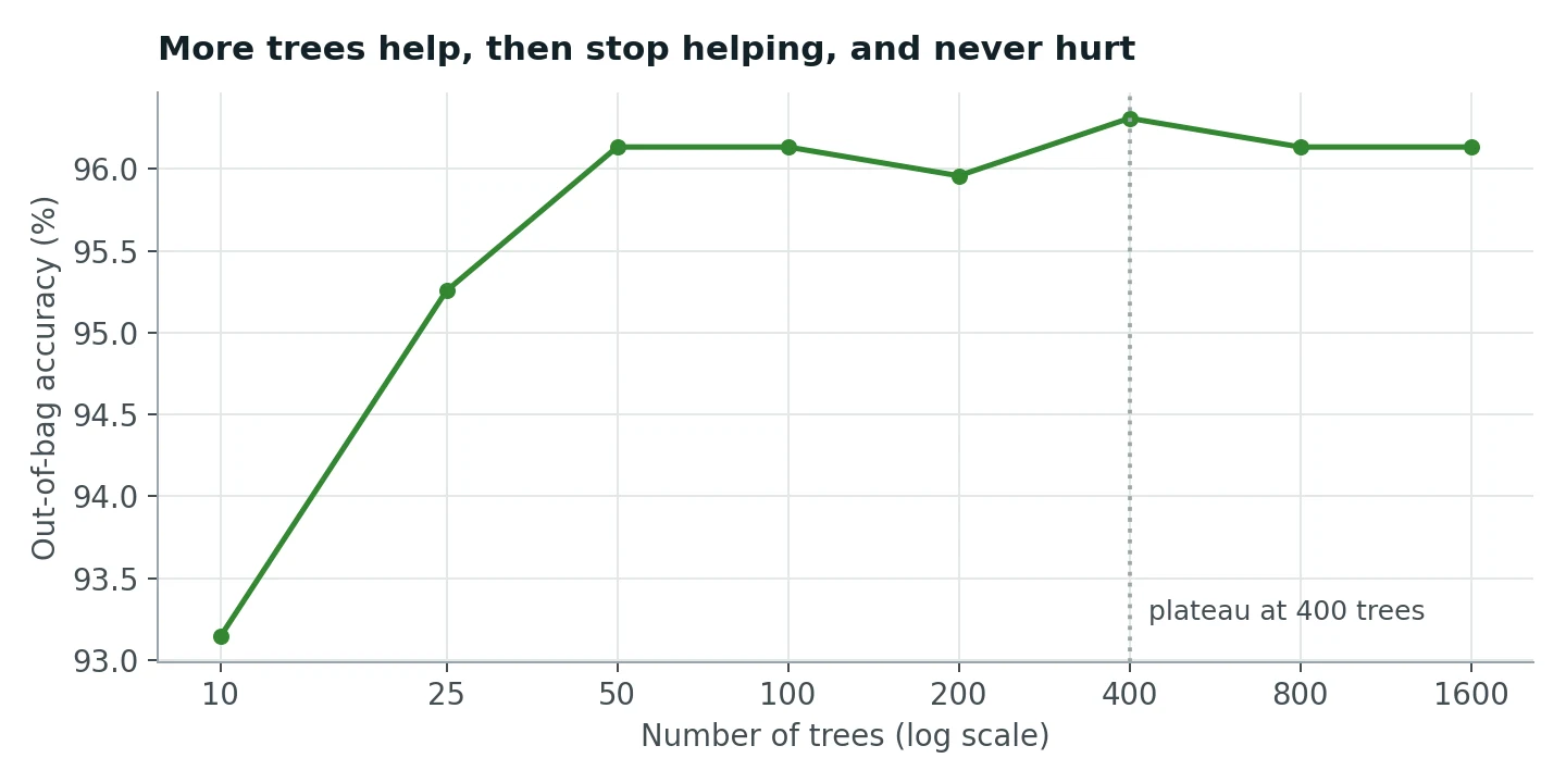
From 10 to 50 trees, OOB accuracy climbs from 93.2% to 96.1%. After that it wobbles between 96.0% and 96.3% all the way to 1,600 trees. Strictly, the peak is at 400 trees (96.3%), but look at the size of the wobble: one tumour out of 569 is worth 0.18 percentage points. The curve is flat from 50 trees onward; everything after that is noise of one or two tumours.
Can more trees hurt? Not accuracy. Adding a tree adds one more vote to an average. It cannot make the forest overfit more, because each tree is independent of the others: the 1,601st tree does not try to fix the mistakes of the first 1,600. (Boosting, which we will meet shortly, is different.) What more trees do cost is training time, memory and prediction latency. So the rule is: add trees until the OOB curve flattens, then stop paying for more.
2. Which features matter? Two methods that disagree#
scikit-learn gives you feature_importances_ for free. This is MDI (mean decrease in impurity): how much each feature reduced Gini impurity, summed over every split in every tree. The alternative is permutation importance: shuffle one column in the test set, breaking its relationship with the label, and measure how much accuracy drops.
from sklearn.inspection import permutation_importance

rf = RandomForestClassifier(n_estimators=500, random_state=42).fit(X_train, y_train)
mdi = rf.feature_importances_
perm = permutation_importance(rf, X_test, y_test, n_repeats=30, random_state=42)
The two rankings barely agree:
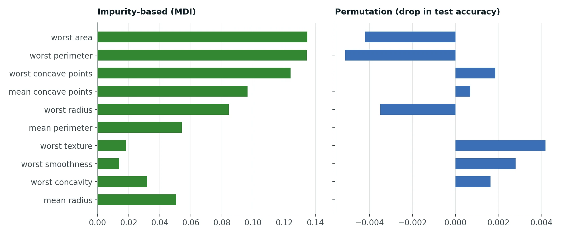
MDI says the most important features are worst area (0.135), worst perimeter (0.135) and worst concave points (0.124). Permutation importance says shuffling worst area or worst perimeter makes no difference at all, and puts worst texture first. Look at the scale, too: the largest permutation importance is 0.004, less than one tumour out of 143.
Is the forest confused? No. The explanation is correlated features. This dataset has nine size-related columns (radius, perimeter and area, each as mean, error and worst), and they are nearly copies of each other: worst radius and worst perimeter correlate at 0.994. Shuffle worst area and the forest simply reads the tumour's size from worst perimeter or worst radius instead. No single size column is irreplaceable, so each one's permutation importance is near zero.
Shuffle all nine size columns together, and test accuracy drops by 28.8 percentage points. Size matters enormously; it is just spread across many redundant columns.
So which would you trust for a clinical report? Neither, on its own:
- MDI is computed on training data and is known to inflate features with many possible split points. But it does credit the size group correctly.
- Permutation importance measures real effect on held-out predictions, which is what you want, but it underrates any feature that has a stand-in.
The practical answer is to group correlated features (by domain knowledge or by clustering the correlation matrix) and compute permutation importance per group. Then report "tumour size" as a single, very important factor, rather than letting the model split the credit nine ways.
3. When the class you care about is rare#
Real screening data is rarely balanced. To simulate that, I kept all 357 benign tumours and only 10% of the malignant ones: 21 malignant cases. Then I compared three approaches:
- A default forest.
- A forest with
class_weight="balanced", which weights each malignant case about 17 times as heavily as a benign one. - The balanced forest, but predicting "malignant" whenever the forest's malignant probability is at least 0.3 instead of the default 0.5.
A first lesson came for free. On a single stratified test split, there were just 6 malignant tumours in the test set, and every model scored a perfect 1.0 on precision, recall and F1. With six positives, one split tells you nothing. So I repeated the experiment 20 times with different random samples of malignant cases, 5-fold cross-validation each time, and pooled the results: 420 malignant predictions in all.
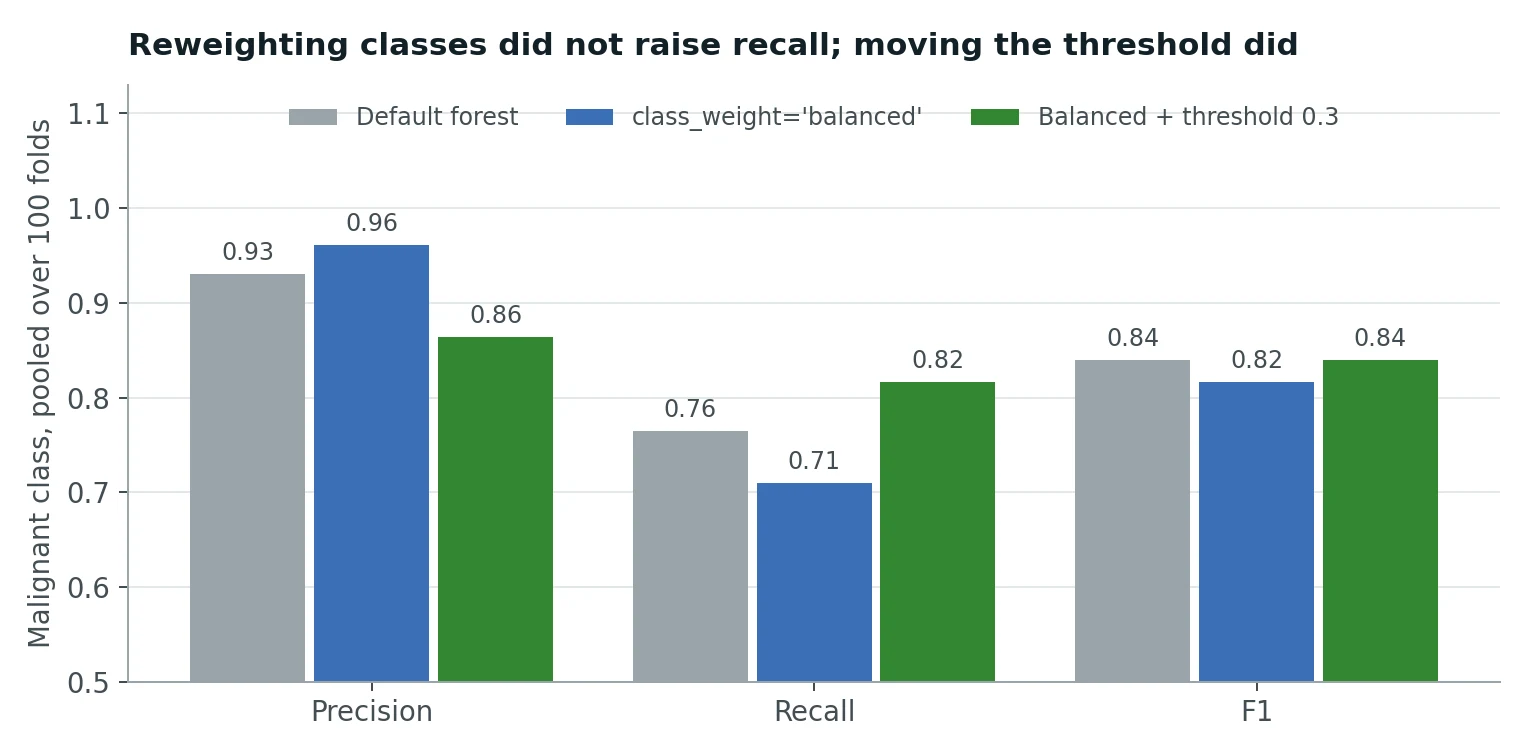
Accuracy was about 98% for all three models, which tells you why accuracy is useless here: a model that called every tumour benign would score 94%.
Look at recall. The textbook fix, class_weight="balanced", lowered it from 0.76 to 0.71. I did not expect that, so I dug in. The culprit is how forests grow by default: every tree keeps splitting until each leaf is pure. Class weights work by changing what a mixed leaf predicts, and a fully grown tree has no mixed leaves. Each of the 17 or so training malignant cases gets fenced into its own tiny pure leaf, weighted or not, and the weights end up shifting which splits are chosen in ways that fence those cases in even more tightly.
To test that explanation, I required every leaf to hold at least 5 samples (min_samples_leaf=5), which forces some leaves to stay mixed. Now the weights have something to act on, and class_weight="balanced" raises recall from 0.72 to 0.79, as the textbook promises. The lesson: class weights and fully grown trees do not mix well.
What actually worked was moving the threshold. At 0.3, recall rose to 0.82: of the 420 malignant cases, the model missed 77 instead of 99. The price was more false alarms (54 benign tumours flagged, against 24), so precision fell to 0.86.
For a cancer screening tool, that is the right trade. A false alarm costs a follow-up test. A missed malignancy can cost a life. Recall on the malignant class is the metric that matters, and the threshold is the most direct dial you have for it. In a real project you would choose the threshold deliberately, for example the highest one that achieves a recall target agreed with clinicians, using a validation set, and then report precision at that recall.
4. Random forest or XGBoost?#
Gradient boosting builds trees sequentially: each new tree is trained to correct the mistakes of the ensemble so far. XGBoost is the best-known implementation. I compared a 400-tree forest with a default XGBClassifier on the same held-out split:
| Random forest | XGBoost | |
|---|---|---|
| Test accuracy | 95.8% | 96.5% |
| Training time (this machine) | 0.37 s | 0.18 s |
| Top feature | worst area | worst radius |
XGBoost is ahead by one tumour, which is not a meaningful difference on 143 test cases. Both are excellent here. Their feature importances also differ in character: the forest spreads credit across the correlated size features (worst area 0.14, worst perimeter 0.13, worst radius 0.08), while XGBoost's gain-based importance concentrates it (worst radius 0.44). Boosting tends to pick one representative of a correlated group and keep using it, which is another reason not to read importances as ground truth.
When to reach for which:
- Random forest when you want a strong result with almost no tuning, when the data is small or noisy, or when you want the free OOB estimate. It is very hard to badly overfit.
- XGBoost (or LightGBM, CatBoost) when you are willing to tune (learning rate, depth, number of rounds, early stopping) in exchange for the last few points of accuracy, which on large tabular datasets are often there to be had. Boosting can overfit with too many rounds, so it needs a validation set.
What to take away#
- A forest averages many deliberately different trees, cutting the variance that makes single trees unreliable.
- Add trees until the OOB curve flattens. More trees never hurt accuracy, only cost.
- MDI and permutation importance answer different questions, and both are distorted by correlated features. Group correlated features before drawing conclusions.
- With a rare class, evaluate over many resamples, not one lucky split, and use the decision threshold, not just class weights, to buy the recall you need.
- Random forests are the dependable default; boosting is the tuned upgrade.